Background – What are Transformers
If you have yet to see it, computer language models (artificial intelligence) has recently exploded in usability, accuracy, and popularity. Models like Google’s Bard, OpenAI’s ChatGPT, Microsoft’s Bing AI, and Claude are all taking over the market for technology today.
These models can do amazing things like provide recipes for dinner, give you ideas for your next Shopify website, build code from the ground up, answer complex theoretical questions, and more. Some models are even adding in support for processing photos, providing links to sources, and even opening up pertinent videos, email, and calendar events. You can try out these models for free, and you can opt in for more powerful version that might cost a premium.
The transformer then is the basic architecture upon which these advanced models are built. Something like Google’s Bard or ChatGPT are a lot more than just a transformer, but it is useful to understand the basics if your are to have any hope of understanding the full production model.
Pre-requisite Knowledge
I throw around the word ‘model’ as if it means something very specific – which in a sense, it does. However, it should be clear that I am not talking about a model as in a a tiny rocketship or a fashionista. Instead, the word ‘model’ in data science often refers to a complex function. Like any function, a model takes an input and it gives back an output. What makes these models special, however, is the degree to which that can distinguish a variety of inputs without having to be specifically coded to do so.
For instance, If I want to take an image and create a function that can tell where an eyeball is in the image, as a programmer, I might first figure out how a circle is represented. I would search the image for circles. Then, I would have to figure out what other parts of the eyeball is distinct from any other circle. You could keep going further using a variety of if-else conditional statements to find out what a circle looks like. However, what if your next image the eyeball is shaped slightly differently? What if it is a different color? What if there is a defect in the eyeball or a reflection inside making it look different? This is where modern neural network style models come in.
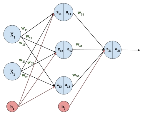
These modern models are not a series of if-else’s, but instead a collection of mathematical operations where the weights of these operations are dynamically changes by the computer using a recursive technique of training with the goal being to minimize the loss (difference) between a target and a prediction. A common representation of a simple neural network (including the weights and biases) is below:
The Transformer
So what exactly is a transformer? The transformer is a series of these neural networks combined in such a way as to be able to keep a representation of inputs from very early on in the text sequence. The transformer architecture that sparked our modern day understanding of large language models came from a paper simply titled ‘Attention Is All You Need.’ This paper – while perhaps not realizing it – sparked the beginning of a large change in AI. The foundational concept of this paper was this idea of attention. Below you can see the encoder-decoder architecture that was proposed in the original paper:
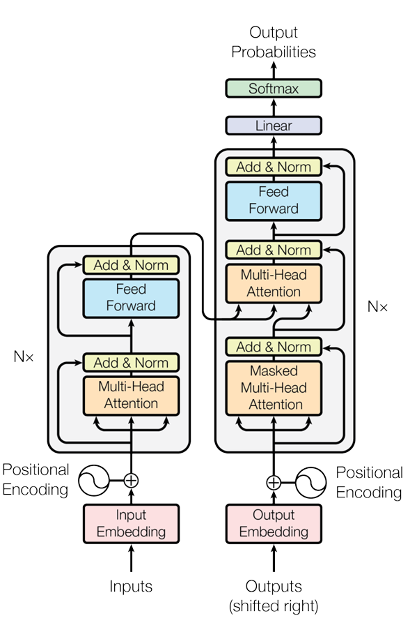
This diagram is very complex and it can seem quite confusing at first, but in this blog post, I am going to break it down. More specifically, I am going to break down the components of the right side of the diagram (the decoder only section).
Attention
This concept of attention derives from one simple concept. This concept is that we want a single word to be able to have reference to what all the other words are around it and how similar it is to those other words. We can find a word’s similarity by calculating a weighted average between a single word and the other words around it. The weights to be chosen can be done as a neural network which we already discussed. However, it is not quite that simple. When you calculate just a weighted average, a lot of information is lost about the original word. We want to be able to retain context, and finding out exactly the right weights can be tricky. The way that we do this then is to take a new set of values from our input and label those as the query. Then we can take those and find out how they relate to each individual word by multiplying it against all the other words in the sentence. To keep our original tokens untouched and to allow for backpropagation, we multiply these queries against another new matrix of values – the keys. Since these new weights are both represented as matrices, to combine them we need to take the dot product.
The queries are represented with a capital Q and the keys with a capital K. To dot product these values, their shapes must be compatible for multiplication, so we have to transpose the Keys – represented as KT. So the dot product is simply Q . KT.
This dot product then represents the weights by which to multiple our original values by in order to find their similarities. However, instead of multiplying them directly, it is better if we can find a relationship from the initial values which represents the specific context a little better. For this reason, we put our initial values through another network to get a matrix of Values – V. These final values can then be multiplied across our new Q . KT weights. to receive out attention scores. However, there is one last adjustment to be made. We want to represent out Q . KT weights as proportional weights (meaning the weights should all add up to 1). This way we are simply taking a weighted average of our Values matrix and not exploding the matrix to much larger values. This con be achieved with the SoftMax function:
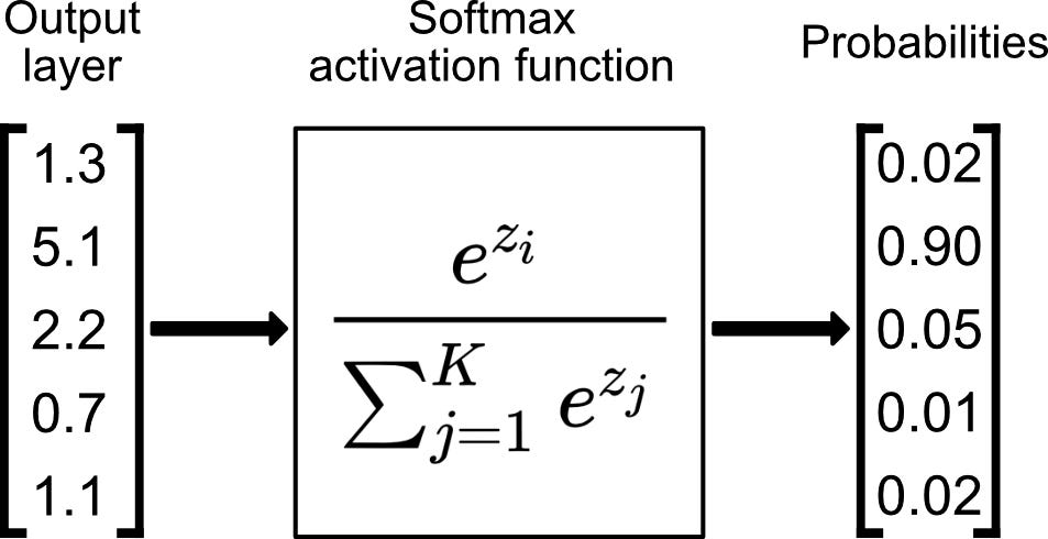
This softmax function, as you can see, weights everything to add together to 1.
This alone, however, still has a problem. if you look in the above image, small values move towards 0 and large values move towards 1. If we end up with a Q . KT weights matrix of a bunch of 0’s and only a single 1, then that is not weighting our values but rather one-hot encoding them. To make sure this doesn’t happen, we want to scale our original Q . KT weights. We can scale them by the dimensionality of our matrices. More specifically, by the square root of the dimensionality of our matrices. In the end, we end up with the following equation:

Multi-Headed Attention
This new mechanism does a great job at finding out the similarities between words or inputs. However, if you consider that one word can have multiple means (e.g. apple being a fruit or a technology company), then it becomes important to realize that we need to calculate different similarities for different contexts. The way attention handles this is with multi-headed attention.
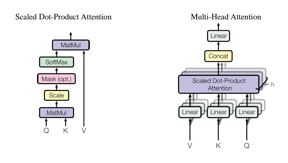
The way multi-headed attention works is that by separating out our input into multiple attention heads (where each head is the formula in figure 4), then each head can worry about understanding similarities under different contexts. These heads can then be concatenated together just like an ensemble model might be. This new concatenation of heads creates a model which can much better predict similarities between words.
Masks
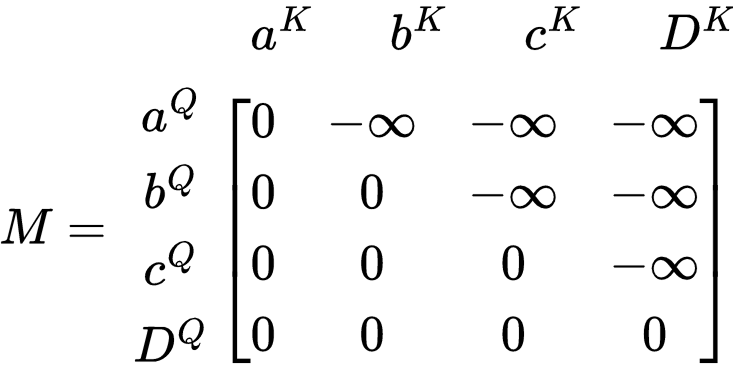
You will notice in figure 5 and in figure 2 there was a word labeled ‘mask’ or ‘masked’ as part of the diagram. What these labels mean is that in some cases, it better for a word to only try to understand the context of all the words that came before it rather than the words that came after it. We can accomplish this by presenting a new matrix which has 1s for each row of input for the column that represents itself and the columns that represent the words before, and you can have 0’s for the columns that represent the words to come after. These 1s can then be represented with the new weights, and the 0’s can be changed to -inf. This way, when the SoftMax equation works on the matrix, the -inf values will go to zero and only the weighted values will be considered for the SoftMax.
Blocks
For even further processing, you can take the multiheaded attention mechanism and chain multiple of them together. In the example from figure 2, this is done so that there can be cross-attention (attention where the queries and keys come from a separate source rather than the input. In this case it comes from the encoder). However, you can still chain blocks even when using purely self attention (the first step of attention in figure 2). These blocks can help to improve the performance of the model slightly.
Adding and Normalizing
With these complexities involved in this process, it becomes very easy for the original inputs to be lost. However, we want the order of the original inputs to be important for the final model (“I ate pizza” and “pizza ate me” are two very different sentences). In order to keep this order, we encode the original values based on their position in the sentence (positional encoding). If we add these positional encodings after each step, then this means that the process of backpropagation (where we train based on loss) can have direct connections to the positions of the words.
There is also a problem in machine learning where values can explode. This means that values can very quickly get bigger and bigger and once they get so big then small changes don’t mean anything. However, small changes of context should have a larger impact in a sentence (imagine “I hate you” versus “I hate your shirt”). In order to prevent this exploding of values, we want to normalize the values to be smaller – i.e. normalize them between 0-1. We can do this with any distribution, but SoftMax works well for this explanation.

Feed Forward and Linear
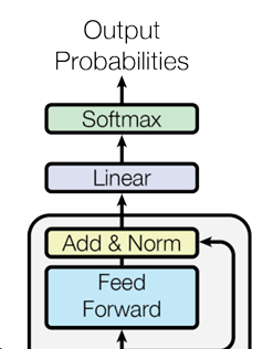
As a last layer, we want to create probability distributions for the probability for what the next word/token will be (token represents a part of a word which is what modern models use instead of full words). In order to do this, we put the final values through a simple neural network like seen in figure 1, then reduce the dimensions to fit the size of our vocabulary so that the size of our dimension is equal to the size of our vocabulary.
These final predictions can then be normalize with SoftMax, and we can use the maximum value in this final distribution to represent the word at that index in the vocabulary. This is our final prediction
The Decoder Only Part
lastly, the part where we make a decoder only transformer is that we start of with our original input and feed it directly into the transformer without giving it an encoder sequence first. The reason for this is that the original paper was trained on translations. This means that if we want to translate “Let’s Go!” into “Vamos!” we want the model to understand the context of “Let’s Go” in it’s final response. However, if we want to just predict words, we can simply feed our words recursively into the decoder portion of the network because we don’t need to keep the attention of the words against a reference at any point.
This means that to use our new network to output a sentence, we would give it some start token, then feed that token through the network, take the output token, and concatenate the output and the start together. This new concatenation can then be refed into the network as many times as you want or until a given stop condition.
Conclusions
All in all this was an introduction to the decoder only architecture that large language models like ChatGPT use to produce useful AI assistants. You can see a project implementing this concept that I created by following along with Andrej Karpathy’s videos here.
These production large language models take this stepping stone and make it much more useful by aligning it to a question answer format, rating response, and using another model to choose the best response in the end. They also train their models on massive datasets with trillions of parameters in the model. You can replicate this on a smaller scale (millions of parameters) but with less successful results.
Hopefully this was a useful introduction, and I encourage you to continue to find out more.